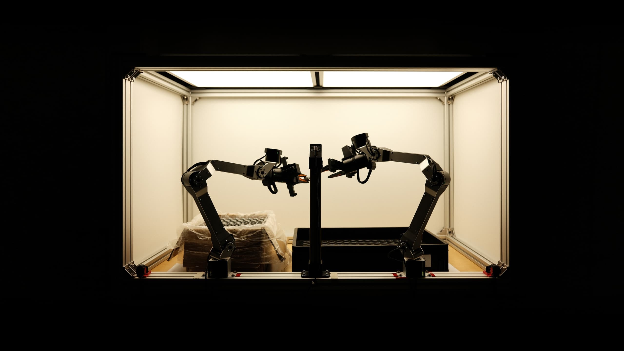
The path to general-purpose robotics runs through task-specific deployments in real workplaces. While much of the field optimises general-purpose policies to do many tasks reasonably well, deployment requires robots that can do one task reliably enough to run unsupervised. At Dream Machines, we focus on closing this gap to 100%, and are model agnostic. This post shares some of our recent results.
The strongest open-source vision-language-action model (VLA) for real-world robotics remains Physical Intelligence’s π0.5[1], which we focus on here. Neither the paper nor the official GitHub repo[2] provides fine-tuning recommendations, and other companies using the model have not published their results.[3] We document our empirical findings from tuning π0.5 on a real-world task from a German manufacturer, with the goal of saving others time adjusting different parameters and informing better data collection.
Task, data & evaluation protocol
1.1The task
Actuators arrive in cardboard boxes and must be transferred into a tray that fixes their position and orientation for a downstream production line. Each actuator must be inserted with its bottom contacts correctly oriented, with both possible 180° rotations acceptable. For these initial experiments, we use only the top layer of the source box: 40 actuators, providing enough diversity and evaluation samples while keeping iteration fast.
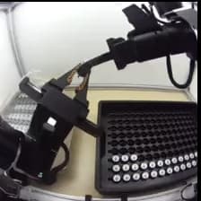
The task requires two arms, both to cover the full workspace and to reorient the actuator for insertion. The left arm picks an actuator from the box and hands it to the right arm, which inserts it into one of the tray’s 135 holes, arranged in 9 rows of 15. The order is fixed: actuators leave the box right to left and bottom to top, and fill the tray left to right and bottom to top. This task is carried out today at a plant of a German manufacturer we are in conversation with. Fig. 1 shows one training episode from the three rig cameras.
1.2Data collection & filtering
We recorded at 50 Hz on bimanual TRLC-DK1[4] workstations using three fisheye cameras (2× wrist, 1× context) at 640×480 pixels in MJPG format. Two teleoperators collected the data using Gello leader arms and a VR headset[5], split evenly across four desks and a lightbox. Data was collected under varying lighting conditions, during the day and at night. The box and tray positions were independently randomised over areas of approximately 11×11 cm. The operators followed the fixed pick-and-place order of Section 1.1 in every episode.
Each episode was rated for quality on a scale from 1 to 5: 1 is an irrecoverable failure, 2 a significant mistake that needed a correction, 3 a minor mistake such as bumping into a neighbouring actuator, 4 a clean episode with a small imperfection, and 5 a clean execution. Fig. 2 shows one calibration clip per rating.
Every episode starts and ends in a rest position. The deployed system will omit this, but we kept it here to simplify the experiments and make them easier to compare.
Preprocessing is minimal: we keep only episodes rated 3 or above, trim idle periods at the start and end, and centre-crop each frame to 224×224, matching the input size of π0.5’s SigLIP encoder. After filtering, the dataset contains 7,271 episodes totalling 21 hours. Every dataset used in this post is public on Hugging Face (Table 3 in the appendix). Fig. 3 shows how the ratings split across the two operators: both rated more than 80% of their episodes 5, and the filter removed fewer than 100 episodes in total. Fig. 4 shows the episode durations after trimming. Most episodes take 8 to 12s, and the two operators are similarly fast.
1.3Evaluation protocol
All evaluations are run in the lightbox, with the boxes at the centre of the randomisation area. Each of the 40 positions in the top layer is evaluated once, giving 40 rollouts per evaluation. In some cases we did multiple evaluation rounds, one round being all 40 actuators in the top layer, to reduce the uncertainty.
Our main metric is the binary success rate. In addition, we recorded the progress of every episode, meaning how far the policy got, in five stages: (1) failed before lifting an actuator, (2) lifted the correct actuator, (3) handed it over cleanly, with the right arm holding it for at least one second, (4) inserted it into the right hole with both edges, but tilted or misoriented, (5) inserted it cleanly with the correct orientation. Each stage requires all previous ones, so lifting the wrong actuator and inserting it into the right hole is a failure, and so is any deviation from the fixed order. Fig. 5 shows one rollout per stage.
A rollout ends after 45s, or earlier if the policy has made no progress for 10s or is visibly stuck in a state it will not recover from. This adds a degree of subjectivity, which we accept. Waiting out a failing policy costs time we would rather spend on trials, and the effect is small next to the noise floor at n = 40.
Evaluations per default run with Real Time Chunking (RTC)[6] enabled, the asynchronous serving scheme from Physical Intelligence in which a new action chunk is generated while the previous one is still executing and blended into it. Section 2.10 describes the settings and varies them. The model’s default hyperparameters are listed in Table 2 in the appendix.
Experiment results
Unless stated otherwise, we fine-tune π0.5 on the full 21 hours of data, with a warmup-stable-decay (WSD) schedule for 50k steps, the last 10k steps of which are quadratically annealed. We set the batch size to 256, following Hugging Face’s shirt folding article[3], and lower the maximum learning rate from 1e-4 to 5e-5, given our different learning rate schedule. Error bars on the success rates below are binomial 95% confidence intervals (CI, Wilson score) over that bar’s n rollouts, about ±15 pp at n = 40. Every chart can be toggled to the progress view, the share of episodes by the furthest stage reached (Section 1.3).
2.1Success plateaued early, and validation error did not tell checkpoints apart
Our first question was simple: how long do you need to fine-tune for?
π0.5 ships with a cosine-decay schedule, which couples the learning rate to the total step budget and makes checkpoints from runs of different lengths hard to compare. We used WSD for a cleaner comparison.
We trained a single model for 210k steps at the stable learning rate, annealing only the last 10k, and evaluated every 10k steps at n = 40. Fig. 6 shows the result: success rate rose sharply up to about 30k steps, then plateaued with strong oscillations. Nothing in it argues for training longer than 30k steps.
Every other run in this post nevertheless trains for 50k steps. Our first pass over these checkpoints, before we traced a confound to gripper plasticity[7] and reran every evaluation, had suggested success still rising at 50k, and we fixed 50k steps with annealing as the budget on that basis. By the time the rerun showed the rise was an artefact, most trainings had started, so we kept the budget rather than redo them. The 76% baseline that anchors the later sections is therefore not a checkpoint of this ladder: it is a separate 50k-step run of the recipe above, with its last 10k steps annealed, evaluated over three rounds (n = 120).
Following Allshire et al.[8], we logged the validation action error (the L2 distance between generated and ground-truth action chunks) on a held-out 5% of the episodes. We find it very useful for seeing when a training run starts to saturate, but as Fig. 7 shows, it does not indicate performance beyond that, most likely because small model differences are not reliably identifiable with our evaluation sample size. An ordinary least squares (OLS) fit of rig success on validation error explains about a fifth of the variance with all checkpoints, and almost none once the two earliest checkpoints, which have both the highest error and the lowest success, are left out. The validation loss, the flow-matching objective on the same held-out episodes, does no better: it rises steadily through the whole run while success stays flat (toggle the x-axis in Fig. 7).
To answer our opening question: in our setting, about 30k steps at batch 256 on 21 hours of data were enough, and neither training longer nor choosing a checkpoint by validation error or loss bought anything a 40-rollout evaluation could see.
2.2LoRA fell well short of full fine-tuning, even at rank 256
Full fine-tuning of π0.5 requires about 37 GB of VRAM and therefore data-centre GPUs. We have RTX 5090s with 32 GB in our office and wondered whether we could train on these. Low-Rank Adaptation (LoRA) only trains small, low-rank adapter matrices to represent weight updates and, at the rank 64 we used, needs only 18 GB. Table 1 shows how that scales with rank. On a 5090 you can technically train with batch size 4 on a compiled model and about 39 when uncompiled[9]. Gradient accumulation turns the batch size that fits into the GPU into any effective batch size (EBS) for gradient updates.
| Rank | Trainable parameters | Peak VRAM |
|---|---|---|
| 16 | 38M (1.1%) | 17.1 GB |
| 32 | 76M (2.3%) | 17.3 GB |
| 64 (ours) | 151M (4.5%) | 17.9 GB |
| 128 | 303M (9.0%) | 18.7 GB |
| 256 (ours) | 605M (18.0%) | 20.7 GB |
| 512 | 1.21B (36.1%) | 30.0 GB |
| Full fine-tune | 3.35B (100%) | about 37 GB before any batch |
Table 1: Trainable parameters and peak VRAM by LoRA rank. LoRA on every linear layer of the vision-language model (VLM) and the action expert, as in our runs. Peak VRAM measured over five training steps at batch 8, uncompiled, with gradient checkpointing, on an RTX 5090. The full fine-tune’s 37 GB is its static cost alone (weights, gradients and AdamW state) and does not include the activations of any batch.
Jon Schulman’s work[10] argues that LoRA can get you the same performance as full fine-tuning on LLMs, provided you apply it to all layers and pick a rank that is able to absorb the information in your data sufficiently. We trained three arms meeting those conditions, all with all-linear targeting[11]. The first keeps our EBS of 256 and takes the recommended 10× learning-rate multiplier (5e-4 vs. our 5e-5 full fine-tune default) at rank 64, which is about 150M trainable parameters against our 21-hour dataset. As Schulman also finds LoRA unable to handle large batch sizes well, the second drops the EBS to 64 and square-root scales the learning rate to 2.5e-4, holding total samples fixed (200k steps vs. 50k). The third keeps that batch size and pushes the rank to 256 (about 600M trainable parameters) to test whether adapter capacity is the binding constraint.
None of them closes the gap (Fig. 8). At rank 64 the EBS-256 arm lands at 45% and the EBS-64 arm at 32.5%, against the full fine-tune’s 76%. The smaller batch made it worse, not better. Rank 256 is the best of the three at 52.5%, still 23 pp below full fine-tuning and right at the edge of what a 40-rollout evaluation can resolve (Section 1.3). Notably, the rank-256 model saw half the samples of the other two (100k steps at batch 64, 6.4M vs. 12.8M)[12]. Rank 256 at an EBS of 256 is the one combination we have not tried, and it would be the natural next LoRA experiment.
We hypothesise that LoRA updates are insufficient because our embodiment is absent from the π0.5 pretraining data: adapting to a new robot is not the small, low-rank edit that LoRA assumes. We did not pursue it further. In the interest of time, training ran on the cloud anyway, and LoRA bought us almost nothing there: the rank-64 EBS-256 arm used about 10% fewer GPU-hours than the full fine-tune, and at a matched EBS of 64 on four H100s the adapter is slower per step than full fine-tuning (0.90 steps/s at rank 64 and 0.65 at rank 256, against 0.95). The adapter saves optimizer memory, not compute.
2.3Low sensitivity to learning rate and batch size in our tested range
Next, we asked how sensitive fine-tuning is to learning rate and batch size. We ran experiments varying both hyperparameters and saw no improvement, nor a statistically significant deterioration (Fig. 9 and Fig. 11). The model seems robust to both settings in our tested range. Batch size 256, as in the Hugging Face post, and our WSD-adjusted learning rate of 5e-5 worked best for us, although the 1e-4 run, which has the lowest success rate of the three, reaches the lowest training loss (Fig. 10). You can hover a bar in Fig. 9 to highlight its loss curve.
2.4Relative joint targets and image augmentation changed nothing
π0.5 predicts absolute joint targets. A common alternative is to predict deltas relative to the current joint state, which re-centres the action distribution around zero and makes it independent of where in the workspace the arm happens to be. We retrained the baseline that way, keeping the grippers absolute[13].
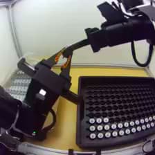
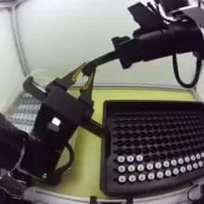
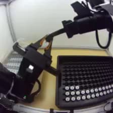
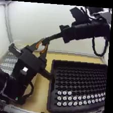
Separately, we tested image augmentation, which our recipe leaves off by default. LeRobot’s default pipeline draws three of its six standard photometric and geometric transforms[14] at random for every frame and applies them in a fixed order, each at a random strength. The appendix shows what each transform does to a training frame (Fig. 26) and what the model sees after the full pipeline (Fig. 27).
Neither made a measurable difference (Fig. 12). Relative joint targets reached 73% and image augmentation 75%, against the baseline’s 76%. Both sit well inside the n = 40 noise floor, so we kept absolute joint targets and no augmentation for all other runs in this post. Note that this is an evaluation in the same setting the data was collected in. Augmentation may still pay off when the deployment scene differs from the training scenes.
2.5Small differences between operators produced very different policies
We evaluated the effect of operator and collection interface by training three models: one on operator 1’s 10h, one on operator 2’s 10h, and one on an equally sampled 10h mix. This comparison confounds operator and interface, as operator 1 used VR teleoperation while operator 2 used Gello leader arms.
The model trained on operator 2’s data underperforms the model trained on operator 1’s data by over 30 pp (Fig. 14), largely due to failed handovers. Once the handover succeeds, the rest of the episode is comparable. The mixed model appears to mostly inherit operator 1’s handover strategy rather than combining both behaviours, which explains why it performs similarly. VR and mixed perform within noise of each other. Notably, operator 2’s handover behaviour results from the Gello arms’ form factor, which forces the operator to reach around them and constrains movements. Fig. 13 shows the two handover styles side by side.
2.6Five times the data lifted success from 63% to 76%
Our goal is to train a deployable policy from one day of data, so we evaluated how performance scales with dataset size. We trained on nested 4h, 10h and 21h subsets of the dataset, each sampled equally across operators and workspaces.
The 4h and 10h models perform similarly, while the 21h model performs better (Fig. 15). However, as the next experiments show, the type of data matters more than the quantity.
2.7Four hours across five scenes beat four hours in the evaluation scene by 30 pp
Shi et al.[15] found that scene diversity matters more than data quantity. We tested this by comparing two 4h models: one trained only on lightbox data (the evaluation setting used throughout all experiments) and one trained on data sampled equally across all four desks, the lightbox and both operators. Fig. 16 shows the five scenes.
The diverse model outperforms the homogeneous one by 30 pp (Fig. 17), despite the latter being trained entirely in the evaluation environment.

2.8One clean hour on 21h bumped performance from 76% to 90%
Most failures occurred during the handover. During teleoperation, we had developed the habit of handing over the actuator very quickly. A common failure was the left gripper releasing before the right had closed, causing the actuator to drop. Recovery episodes picking the actuator back up were labelled 2, so our grade-3-to-5 filter removed exactly the required recovery behaviour, and a handover failure virtually always meant a trial failure. We also found that many episodes labelled as clean were not completely flawless.
To test the effect of data quality, we collected one additional hour in the lightbox under strict constraints: consistent motion throughout and insertions that cleared the tray edges (Fig. 18). This meant that the mean episode length roughly doubled. We used it in two ways, fine-tuning π0.5 from scratch on only this data for 10k steps, and continuing training from our 21h/50k checkpoint for 5k more steps, annealing the last thousand, at a reduced learning rate of 2e-5.
Fine-tuning the 21h policy on this hour improved success from 76% to 90% (Fig. 19). Training from the π0.5 base model on this hour alone reached 28%, within 5 pp of the 4h lightbox-only model despite using only a quarter as much data. While still well below the 4h diverse model, it strongly supported the ML adage that data quality matters more than quantity.
2.9240 rollouts with interventions took a 1h policy from 28% to 88%
Dataset aggregation (DAgger)-style data collection is one of the few methods that have been replicated and consistently shown to improve policy performance. Motivated by the results in the previous section, we wondered how far we could get with a small high-quality dataset and added human-gated intervention data[16] to our 1h dataset. We started from the 1h-from-scratch policy rather than from the 21h + 1h model on purpose: the question was how much performance a minimal amount of data can buy.
We rolled out the 1h-from-scratch policy for 240 episodes, clearing the top tray six times, and intervened whenever the policy was about to make a mistake. For the first tray, we placed the boxes in the evaluation orientation. For the remaining trays, we varied their position and orientation as during data collection. Of the 240 episodes, 212 included interventions. For the next training run, we used only the intervention segments from these episodes, along with the full trajectories of the remaining 28 successful episodes. Combined with the initial 1h dataset, this yielded 1.7 hours of training data.
Fine-tuning on this data increased success from 28% to 88% on the standard evaluation setup (Fig. 20). To test whether this improvement was position-specific, we also evaluated on more diverse box positions, where success increased from 11% to 48%. Notably, this model trained on just 1.7 hours of data outperforms the model trained on 21h of data by 12 pp. It should be noted though that all of the 1.7 hours were collected in the lightbox, which was also the evaluation setting of both models.
2.10Serving settings alone took the same checkpoint from 76% to 93%
Seeing the handover failures, we asked whether the problem was that the model had to commit to a handover while the arms were still far apart. We had first hypothesised that the handover motions were simply too fast to learn, but the slower data of Section 2.8 fixed most of these failures, which points at the prediction horizon instead: with slower motions, by the time the model predicts the handover, both end effectors are already close to one another.
We wondered whether we could achieve a similar gain by changing the RTC settings. Our setup runs at 50 Hz with an action chunk of 50 actions (1s). Two settings govern the schedule. reinfer is the number of actions left in the queue when the next chunk is requested, and blend is how many of the new chunk’s first actions are guided towards the overlapping actions of the previous chunk. Our default so far was reinfer = 30 and blend = 16. Inference takes about 140ms, so the first seven actions of a new chunk are already in the past when it arrives and are executed from the old chunk regardless. reinfer = 50 therefore behaves like reinfer = 43. Fig. 21 lets you play with these settings[17].
A new chunk is requested when 30 actions remain in the queue and arrives 7 ticks later, with 23 of them still queued. Of its 50 actions, the first 7 are frozen to the old chunk, the next 9 are blended towards it and the remaining 34 are free.
Changing the reinference frequency had little effect, although more frequent reinference performed slightly better by making the policy more reactive (Fig. 22). Blend mattered much more: with immediate reinference, a blend of 20 achieved the best result, increasing success to 93%. Applying these settings to the 21h + 1h model from Section 2.8 improved its performance further, from 90% to 98%, with only one failure in 40 trials. We also compiled the model to shorten the inference delay, so that reinference happens even more often. This didn’t help. The compiled arm in Fig. 22 lands below its uncompiled twin. It appears that beyond a point, reinferring faster may not buy much.
The intervention model of Section 2.9 is not part of this comparison. The two experiments ran in parallel, so it was never served with the improved settings.
Together with Section 2.8, this supports the idea that the model struggles to predict movements when the arms are farther apart: both more frequent predictions and slower movements shrink the distance the arms travel between observations, so the handover is predicted with the arms closer together.
An obvious next step would be to combine the 21h data, the high-quality hour, the intervention data and the best RTC settings in one model. With 40 rollouts per evaluation, though, the result would be too noisy to support a meaningful statement, so we turned to one final question instead.
2.11Without the pretrained π0.5 weights, not a single insertion succeeded
The π0 paper[18] included a result showing fine-tuning from pretrained checkpoints only marginally outperformed training from scratch. We therefore tested whether π0.5 could also be trained from scratch, initialising only the PaliGemma backbone. Since π0.5, Physical Intelligence has not released new weights but has substantially changed the architecture (a newer Gemma backbone, 2× higher image resolution, and a 2× larger diffusion head). If the performance gap remained similarly small, these architectural improvements could potentially outweigh the lack of pretraining.
The resulting policy produces plausible motions (Fig. 24) but fails to complete a single insertion (Fig. 25). 7 of 40 evaluations fail to grasp the correct actuator (or any actuator), 29 of the remaining 33 fail during the handover and the last 4 during insertion. Notably, the handover mode resembles the one of operator 2, which was associated with worse performance in our operator experiment. Although based on a single task, this suggests pretrained π0.5 weights are far more important than the π0 results implied.
Takeaways & limitations
Our main takeaways for future experiments are to optimise for scene diversity rather than pure data quantity, to keep teleoperating fast where it makes sense but to move slowly right before steps that require precision, so that critical action chunks are predicted from close observations, and, instead of collecting a big dataset straight away, to start with a small amount of data, train a simple policy, and then improve it with intervention data or with additional demonstrations of the situations in which it fails.
A clear limitation of these experiments is that all results are from a single task. We also examined hyperparameters individually rather than in combination, even though their effects certainly interact. And a general limitation of real-world robotics is that evaluations are slow and noisy due to the small sample size. We are sharing these results nevertheless, given how few experience reports on making policies work in the real world exist.
A few questions stayed open for lack of time, but might be interesting for others to look at. Is a context camera necessary? Can black-pixel padding of our 4:3 images match or beat square cropping? Can the number of flow-matching steps be reduced for faster inference, or raised for better performance, without a loss elsewhere? Would longer annealing help? And could two-stage training, first on all quality ratings and then only on the high-quality episodes, yield a policy that executes cleanly yet still recovers from failures?
What’s next
As we approach 100% success on the top layer, distinguishing between policies from rollouts alone becomes increasingly difficult. The remaining differences are smaller than what 40 evaluations can reliably resolve. So we are moving to the full box, matching the task exactly as it runs in production.
Imitation learning is an effective way to acquire a skill, but it has a ceiling. Closing the gap to 100% cannot come from a human closing data gaps or tuning hyperparameters. It requires the model to learn from its own experience. A policy should not just recover from failures, but become faster at doing so and learn how to avoid them completely. We see closing that gap as a reinforcement learning problem, and that is where our focus is shifting next.
If this sounds interesting to you and you’re the kind of person who’s comfortable moving between arXiv and the factory floor, then let’s have a chat. d@dream-machines.eu. We’re hiring.
Appendix
Architectural and training defaults from the reference YAML and paper (Table 2). These do not vary across experiments unless stated otherwise.
| Parameter | Value | Note |
|---|---|---|
chunk_size | 50 | action horizon: 1s at 50 Hz |
n_action_steps | 50 | full chunk executed before re-query |
n_obs_steps | 1 | single observation timestep |
num_inference_steps | 10 | flow-matching denoising steps |
image_resolution | [224, 224] | SigLIP input size |
tokenizer_max_length | 200 | π0.5 default (π0 used 48) |
normalization | QUANTILES | state + action, robust to outliers |
time_sampling | Beta(α = 1.5, β = 1.0) | flow-matching timestep distribution |
dtype | bfloat16 | required to fit the 3B-parameter VLM |
Table 2: Default settings
Image augmentation, as tested in Section 2.4: LeRobot’s six default transforms, three of which are drawn per frame and applied in a fixed order. Fig. 26 shows each transform alone, drawn near the strong end of its range, and Fig. 27 shows five random draws of the full pipeline on the same frame.
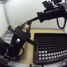
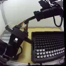
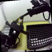
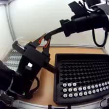
Every training dataset used in this post is public on Hugging Face, in LeRobot format (Table 3). Hours are frames at 50 Hz.
| Dataset | Episodes | Hours | Used in |
|---|---|---|---|
| actuator_unboxing_20h_345 | 7,271 | 21.4 | 2.1 (210k-step ladder), 2.2 (rank 64 at EBS 256) |
| actuator_unboxing_20h_345_v2 | 7,271 | 21.0 | 2.1 (50k baseline), 2.2 (both EBS-64 arms), 2.3, 2.4, 2.6 (21h), 2.10, 2.11 |
| actuator_unboxing_10h_vr | 3,460 | 9.8 | 2.5 (operator 1) |
| actuator_unboxing_10h_leaderarms | 3,253 | 9.5 | 2.5 (operator 2) |
| actuator_unboxing_10h_diverse | 3,368 | 9.7 | 2.5 (mixed), 2.6 (10h) |
| actuator_unboxing_4h_diverse | 1,344 | 3.9 | 2.6 (4h), 2.7 (five scenes) |
| actuator_unboxing_4h_lightbox | 1,569 | 4.0 | 2.7 (lightbox only) |
| actuator_unboxing_1h_HQ | 198 | 1.0 | 2.8 (both arms), 2.9 (base policy) |
| actuator_unboxing_1h_HQ_dagger_intv | 512 | 1.7 | 2.9 (the hour above plus the intervention segments of 240 rollouts) |
Table 3: Training datasets on Hugging Face. The two 21h sets hold the same 7,271 episodes; v2 is the export used everywhere except the two earlier runs listed against the first. The relative-joint-target arm of Section 2.4 trained on a local re-export of v2 with actions as deltas, which was not uploaded. Evaluation rollouts are not included.
Notes
1.RoboDojo real-world leaderboard, as of August 2026.
2.github.com/Physical-Intelligence/openpi
3.The only high-quality resource, to the best of our knowledge, is Hugging Face’s Unfolding Robotics blog post.
4.github.com/robot-learning-co/trlc-dk1
5.We also open-sourced the VR teleop kit on GitHub.
6.Black et al., “Real-Time Execution of Action Chunking Flow Policies”, Physical Intelligence, 2025: arxiv.org/abs/2506.07339
7.Find more details here.
8.Allshire et al., “Scalable Behavior Cloning with Open Data, Training, and Evaluation”, 2026: abc.bot
9.Memory and speed numbers are from our single-GPU π0.5 benchmark across six GPU types (RTX 5090, RTX PRO 6000, A100-40/80, H100, H200).
10.Schulman et al., “LoRA Without Regret”, Thinking Machines, Sep 2025: thinkingmachines.ai/blog/lora
11.The adapter’s scaling factor lora_alpha was 32 in all three arms. LoRA multiplies the adapter update by α/r, alpha divided by the rank, so hold alpha fixed when changing the rank. Our first rank-256 attempt scaled alpha with the rank to 128, keeping α/r constant, which under Adam multiplies the effective step on the adapter by roughly √(r₁/r₀). Its gradient norm grew exponentially from about 110k steps and the run was abandoned. Rank 256 at alpha 32 trained cleanly.
12.We stopped the rank-256 run at 100k steps. Its validation action error had saturated, and spending twice the compute on a run that had clearly plateaued did not seem worth it.
13.A delta is taken against the measured gripper opening, and a gripper holding a part never reads as closed, so a zero delta would mean “hold at the part’s width” and release the squeeze, whereas “fully closed” is the same command whatever is in the gripper.
14.LeRobot’s default image_transforms: brightness, contrast, saturation and hue jitter, a sharpness jitter, and a small random affine (±5°, 5% translation). Three of the six are drawn per frame and applied in that fixed order.
15.Shi et al., “Is Diversity All You Need for Scalable Robotic Manipulation?”, 2025: arxiv.org/abs/2507.06219
16.For more experiments on human-in-the-loop data collection see Arnold, “Human-in-the-Loop Data Collection”, 2026: aurelarnold.xyz
17.A simplification: the tool treats the predicted and the actual inference delay as the same number and gives every chunk the same delay. RTC sizes the frozen prefix from a delay estimate, and the real delay varies from chunk to chunk.
18.Black et al., “π0: A Vision-Language-Action Flow Model for General Robot Control”, Physical Intelligence, 2024, Figure 11: arxiv.org/abs/2410.24164